TA的每日心情 | 开心
2019-8-9 09:22 |
|---|
签到天数: 18 天 连续签到: 1 天 [LV.4]偶尔看看III 累计签到:18 天
连续签到:1 天
|
 发表于 2013-3-27 11:12:47
|
显示全部楼层
发表于 2013-3-27 11:12:47
|
显示全部楼层
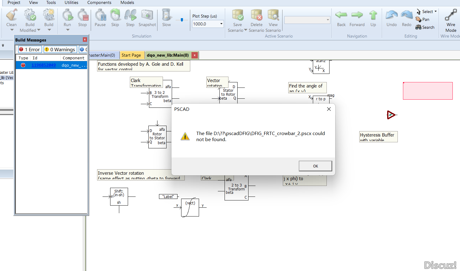
The Bergeron and Frequency Dependent line models are based on traveling wave theory, and thus have a limitation on the minimum length where they can be used (i.e. the travel time must be >= the time step). For a time step of 50 ms, this length is about 15 km. For lines shorter than this, a PI Section model is more suitable.+ Q* h2 ^2 I- [2 D3 \+ g, X8 f: g
% i; ]) s% q$ n) N' q& A
When the traveling wave line models are used, the calculated travel time of the line/cable will not be an exact integer multiple of the time step. The user is given a choice to interpolate the travel time or not. Not interpolating the travel time can introduce errors by artificially increasing or decreasing the effective line length. Interpolating the travel time will give the correct effective length (and the correct fundamental impedance), but has the disadvantage that it adds additional damping at high frequencies. For example, an open ended loss-less line with a step input should result in the open-end voltage stepping from 0 to 2 forever. If interpolation of the travel time is chosen, the square wave will eventually lose all high frequency components and become more of a sine wave |
|


 狗仔卡
狗仔卡 提升卡
提升卡 置顶卡
置顶卡 沉默卡
沉默卡 喧嚣卡
喧嚣卡 变色卡
变色卡 显身卡
显身卡